
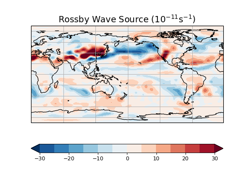
Rossby wave source
(Source code, png, hires.png, pdf)

"""Compute Rossby wave source from the long-term mean flow.

This example uses the xarray interface.

Additional requirements for this example:

* xarray (http://xarray.pydata.org)
* matplotlib (http://matplotlib.org/)
* cartopy (http://scitools.org.uk/cartopy/)

"""
import cartopy.crs as ccrs
import matplotlib as mpl
import matplotlib.pyplot as plt
import xarray as xr

from windspharm.xarray import VectorWind
from windspharm.examples import example_data_path

mpl.rcParams['mathtext.default'] = 'regular'


# Read zonal and meridional wind components from file using the xarray module.
# The components are in separate files.
ds = xr.open_mfdataset([example_data_path(f)
                        for f in ('uwnd_mean.nc', 'vwnd_mean.nc')])
uwnd = ds['uwnd']
vwnd = ds['vwnd']

# Create a VectorWind instance to handle the computations.
w = VectorWind(uwnd, vwnd)

# Compute components of rossby wave source: absolute vorticity, divergence,
# irrotational (divergent) wind components, gradients of absolute vorticity.
eta = w.absolutevorticity()
div = w.divergence()
uchi, vchi = w.irrotationalcomponent()
etax, etay = w.gradient(eta)
etax.attrs['units'] = 'm**-1 s**-1'
etay.attrs['units'] = 'm**-1 s**-1'

# Combine the components to form the Rossby wave source term.
S = eta * -1. * div - (uchi * etax + vchi * etay)

# Pick out the field for December at 200 hPa.
S_dec = S[S['time.month'] == 12]

# Plot Rossby wave source.
clevs = [-30, -25, -20, -15, -10, -5, 0, 5, 10, 15, 20, 25, 30]
ax = plt.subplot(111, projection=ccrs.PlateCarree(central_longitude=180))
S_dec *= 1e11
fill = S_dec[0].plot.contourf(ax=ax, levels=clevs, cmap=plt.cm.RdBu_r,
                              transform=ccrs.PlateCarree(), extend='both',
                              add_colorbar=False)
ax.coastlines()
ax.gridlines()
plt.colorbar(fill, orientation='horizontal')
plt.title('Rossby Wave Source ($10^{-11}$s$^{-1}$)', fontsize=16)
plt.show()