"""
Compute streamfunction and velocity potential from the long-term-mean
flow.
This example uses the xarray interface.
Additional requirements for this example:
* xarray (http://xarray.pydata.org)
* matplotlib (http://matplotlib.org/)
* cartopy (http://scitools.org.uk/cartopy/)
"""
import cartopy.crs as ccrs
import matplotlib as mpl
import matplotlib.pyplot as plt
import xarray as xr
from windspharm.xarray import VectorWind
from windspharm.examples import example_data_path
mpl.rcParams['mathtext.default'] = 'regular'
# Read zonal and meridional wind components from file using the xarray module.
# The components are in separate files.
ds = xr.open_mfdataset([example_data_path(f)
for f in ('uwnd_mean.nc', 'vwnd_mean.nc')])
uwnd = ds['uwnd']
vwnd = ds['vwnd']
# Create a VectorWind instance to handle the computation of streamfunction and
# velocity potential.
w = VectorWind(uwnd, vwnd)
# Compute the streamfunction and velocity potential.
sf, vp = w.sfvp()
# Pick out the field for December.
sf_dec = sf[sf['time.month'] == 12]
vp_dec = vp[vp['time.month'] == 12]
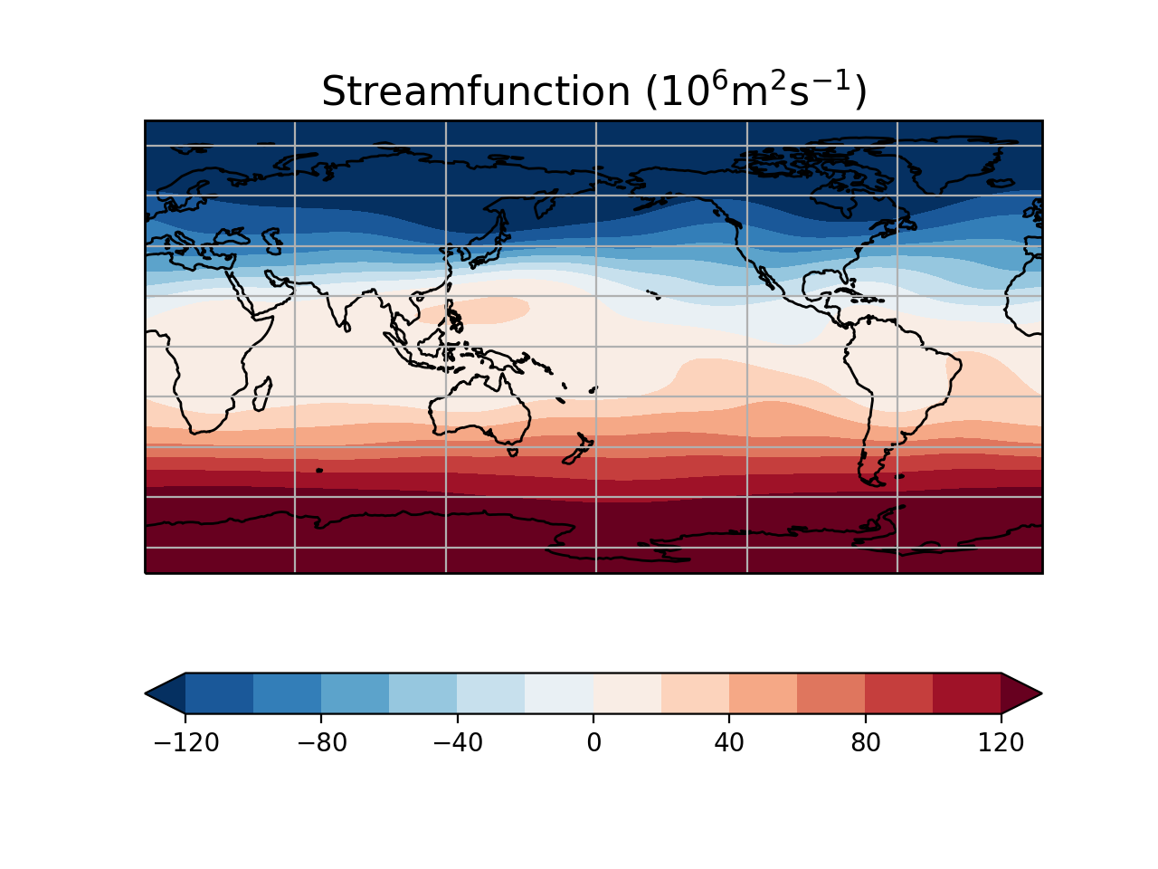
# Plot streamfunction.
clevs = [-120, -100, -80, -60, -40, -20, 0, 20, 40, 60, 80, 100, 120]
ax = plt.subplot(111, projection=ccrs.PlateCarree(central_longitude=180))
sf_dec *= 1e-6
fill_sf = sf_dec[0].plot.contourf(ax=ax, levels=clevs, cmap=plt.cm.RdBu_r,
transform=ccrs.PlateCarree(), extend='both',
add_colorbar=False)
ax.coastlines()
ax.gridlines()
plt.colorbar(fill_sf, orientation='horizontal')
plt.title('Streamfunction ($10^6$m$^2$s$^{-1}$)', fontsize=16)
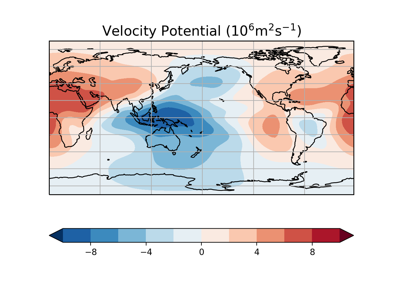
# Plot velocity potential.
plt.figure()
clevs = [-10, -8, -6, -4, -2, 0, 2, 4, 6, 8, 10]
ax = plt.subplot(111, projection=ccrs.PlateCarree(central_longitude=180))
vp_dec *= 1e-6
fill_vp = vp_dec[0].plot.contourf(ax=ax, levels=clevs, cmap=plt.cm.RdBu_r,
transform=ccrs.PlateCarree(), extend='both',
add_colorbar=False)
ax.coastlines()
ax.gridlines()
plt.colorbar(fill_vp, orientation='horizontal')
plt.title('Velocity Potential ($10^6$m$^2$s$^{-1}$)', fontsize=16)
plt.show()


