"""
Compute streamfunction and velocity potential from the long-term-mean
flow.
This example uses the standard interface.
Additional requirements for this example:
* netCDF4 (http://unidata.github.io/netcdf4-python/)
* matplotlib (http://matplotlib.org/)
* cartopy (http://scitools.org.uk/cartopy/)
"""
import cartopy.crs as ccrs
from cartopy.mpl.ticker import LongitudeFormatter, LatitudeFormatter
from cartopy.util import add_cyclic_point
import matplotlib as mpl
import matplotlib.pyplot as plt
from netCDF4 import Dataset
from windspharm.standard import VectorWind
from windspharm.tools import prep_data, recover_data, order_latdim
from windspharm.examples import example_data_path
mpl.rcParams['mathtext.default'] = 'regular'
# Read zonal and meridional wind components from file using the netCDF4
# module. The components are defined on pressure levels and are in separate
# files.
ncu = Dataset(example_data_path('uwnd_mean.nc'), 'r')
uwnd = ncu.variables['uwnd'][:]
lons = ncu.variables['longitude'][:]
lats = ncu.variables['latitude'][:]
ncu.close()
ncv = Dataset(example_data_path('vwnd_mean.nc'), 'r')
vwnd = ncv.variables['vwnd'][:]
ncv.close()
# The standard interface requires that latitude and longitude be the leading
# dimensions of the input wind components, and that wind components must be
# either 2D or 3D arrays. The data read in is 3D and has latitude and
# longitude as the last dimensions. The bundled tools can make the process of
# re-shaping the data a lot easier to manage.
uwnd, uwnd_info = prep_data(uwnd, 'tyx')
vwnd, vwnd_info = prep_data(vwnd, 'tyx')
# It is also required that the latitude dimension is north-to-south. Again the
# bundled tools make this easy.
lats, uwnd, vwnd = order_latdim(lats, uwnd, vwnd)
# Create a VectorWind instance to handle the computation of streamfunction and
# velocity potential.
w = VectorWind(uwnd, vwnd)
# Compute the streamfunction and velocity potential. Also use the bundled
# tools to re-shape the outputs to the 4D shape of the wind components as they
# were read off files.
sf, vp = w.sfvp()
sf = recover_data(sf, uwnd_info)
vp = recover_data(vp, uwnd_info)
# Pick out the field for December and add a cyclic point (the cyclic point is
# for plotting purposes).
sf_dec, lons_c = add_cyclic_point(sf[11], lons)
vp_dec, lons_c = add_cyclic_point(vp[11], lons)
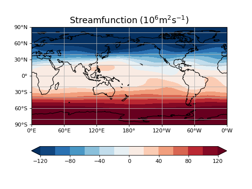
# Plot streamfunction.
ax1 = plt.axes(projection=ccrs.PlateCarree(central_longitude=180))
clevs = [-120, -100, -80, -60, -40, -20, 0, 20, 40, 60, 80, 100, 120]
sf_fill = ax1.contourf(lons_c, lats, sf_dec * 1e-06, clevs,
transform=ccrs.PlateCarree(), cmap=plt.cm.RdBu_r,
extend='both')
ax1.coastlines()
ax1.gridlines()
ax1.set_xticks([0, 60, 120, 180, 240, 300, 359.99], crs=ccrs.PlateCarree())
ax1.set_yticks([-90, -60, -30, 0, 30, 60, 90], crs=ccrs.PlateCarree())
lon_formatter = LongitudeFormatter(zero_direction_label=True,
number_format='.0f')
lat_formatter = LatitudeFormatter()
ax1.xaxis.set_major_formatter(lon_formatter)
ax1.yaxis.set_major_formatter(lat_formatter)
plt.colorbar(sf_fill, orientation='horizontal')
plt.title('Streamfunction ($10^6$m$^2$s$^{-1}$)', fontsize=16)
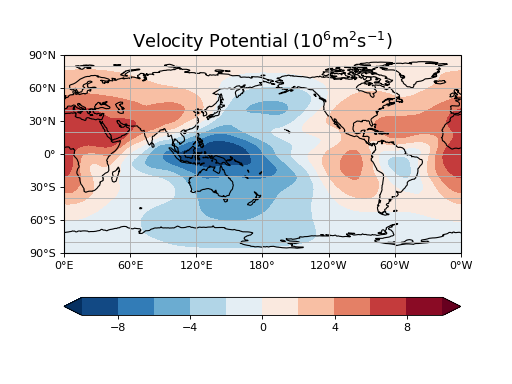
# Plot velocity potential.
plt.figure()
ax2 = plt.axes(projection=ccrs.PlateCarree(central_longitude=180))
clevs = [-10, -8, -6, -4, -2, 0, 2, 4, 6, 8, 10]
vp_fill = ax2.contourf(lons_c, lats, vp_dec * 1e-06, clevs,
transform=ccrs.PlateCarree(), cmap=plt.cm.RdBu_r,
extend='both')
ax2.coastlines()
ax2.gridlines()
ax2.set_xticks([0, 60, 120, 180, 240, 300, 359.99], crs=ccrs.PlateCarree())
ax2.set_yticks([-90, -60, -30, 0, 30, 60, 90], crs=ccrs.PlateCarree())
lon_formatter = LongitudeFormatter(zero_direction_label=True,
number_format='.0f')
lat_formatter = LatitudeFormatter()
ax2.xaxis.set_major_formatter(lon_formatter)
ax2.yaxis.set_major_formatter(lat_formatter)
plt.colorbar(vp_fill, orientation='horizontal')
plt.title('Velocity Potential ($10^6$m$^2$s$^{-1}$)', fontsize=16)
plt.show()


